Final Project: Comparative Analysis of Fuel Efficiency in Various Vehicle Types - LIS 4273

 

Final Project: Comparative Analysis of Fuel Efficiency in Various Vehicle Types

Step 1: Choosing a Dataset

Dataset: Fuel Economy Data from the US Department of Energy (http://www.fueleconomy.gov/feg/download.shtm)

 

Step 2: Sampling and Hypothesis

Sample Size: 250 vehicles

Null Hypothesis (H0): There is no significant difference in fuel efficiency between different vehicle types.

Alternative Hypothesis (H1): There is a significant difference in fuel efficiency (MPG/City) between different vehicle types.

 

Step 3: Write-up Summary

This study aims to determine whether different types of vehicles have statistically significant differences in fuel efficiency. Customers place a high value on fuel economy, and knowledge about the capabilities of various car models can help lawmakers and consumers alike.

This study is consistent with what was discussed in class on analysis of variance (ANOVA) and hypothesis testing. The groundwork for choosing suitable statistical techniques to evaluate the differences in fuel efficiency between various car models has been laid by previously discussed subjects in class.

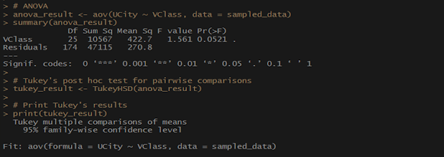
I will utilize an ANOVA to answer the study question. An analysis of variances in fuel economy between different types of vehicles can be done effectively with ANOVA since it permits the comparison of means across numerous groups. The type of vehicle (compact, SUV, etc.) is the categorical variable, and fuel efficiency is the continuous variable.

The following R code was used to conduct the ANOVA variance analysis:

Step 4: Generate Visualization and Abstract

Visualization

To show the distribution of fuel efficiency for each type of vehicle, I created a boxplot. A clear comparison of the fuel efficiency distribution and central tendency across different vehicle types was made possible by this graphical approach.

The purpose of this study is to determine whether there are any statistically significant differences in fuel efficiency across different vehicle classes using ANOVA. The boxplot provides insights into the possible effects on customers and the car industry by graphically illustrating the difference in fuel efficiency. The results will advance our knowledge of how different car models differ in terms of fuel efficiency, which will have consequences for consumer decisions as well as environmental concerns.

Module #12 Assignment

Module #18 Assignment

R's plot() function can be used to show the data. You can plot the values from each year separately or overlay them for comparison because you have data from two years.

credit_card_data <- data.frame(

  Month = c("Jan", "Feb", "Mar", "Apr", "May", "Jun", "Jul", "Aug", "Sep", "Oct", "Nov", "Dec"),

  Year_2012 = c(31.9, 27, 31.3, 31, 39.4, 40.7, 42.3, 49.5, 45, 50, 50.9, 58.5),

  Year_2013 = c(39.4, 36.2, 40.5, 44.6, 46.8, 44.7, 52.2, 54, 48.8, 55.8, 58.7, 63.4)

)

plot(credit_card_data$Month, credit_card_data$Year_2012, type = "l", col = "blue", ylim = range(credit_card_data$Year_2012, credit_card_data$Year_2013), xlab = "Month", ylab = "Credit Card Charges", main = "Credit Card Charges Over Time")

lines(credit_card_data$Month, credit_card_data$Year_2013, col = "red")

legend("topright", legend = c("2012", "2013"), col = c("blue", "red"), lty = 1)

b. The R ets() function, which stands for error, trend, and seasonality, can be used for the Exponential Smoothing Model. This is a basic example:

ts_data <- ts(cbind(credit_card_data$Year_2012, credit_card_data$Year_2013), start = c(2012, 1), frequency = 12)

model <- ets(ts_data)

summary(model)

c. You can see how credit card charges have changed over the course of the months in both years by looking at the time series plot. The fitted model's characteristics, such as the error, trend, and seasonality components, are detailed in the Exponential Smoothing Model summary. You can talk about any conclusions you draw from the time series plot, including trends, patterns, and insights. Furthermore, by using the patterns found in the findings of the Exponential Smoothing Model, you can forecast future credit card charges and gain insight into the underlying elements.

Module 11 Assignment

 Module 11 Assignment

Question 10.1: Set up an additive model for the ashina data

Using the R ISwR package, you can build up an additive model for the ashina data. You can set up the model using the following:

library(ISwR)

data(ashina)

ashina$subject <- factor(1:16)

attach(ashina)

act <- data.frame(vas = vas.active, subject, treat = 1, period = grp)

plac <- data.frame(vas = vas.plac, subject, treat = 0, period = grp)

After preparing your data, you can now build up your additive model and evaluate the impact of subjects, periods, and treatments by comparing the outcomes with t-tests.

Question 10.3: Generate model matrices for models z ~ a*b, z ~ a:b, etc.

The task at hand involves creating model matrices for various models by utilizing the vectors a, b, x, y, and z. It is necessary to conduct out the model fits and talk about the consequences of each model. You can use the following:

a <- c(2, 2, 8)

b <- c(2, 4, 8)

x <- 1:8

y <- c(1:4, 8:5)

z <- rnorm(8)

model_matrix_a_b <- model.matrix(~a * b)

model_matrix_a_colon_b <- model.matrix(~a:b)

lm_a_b <- lm(z ~ model_matrix_a_b)

lm_a_colon_b <- lm(z ~ model_matrix_a_colon_b)

After creating model matrices for the models z ~ a * b and z ~ a:b, you have fitted linear models to the given data. These models' outputs can be compared, and their ramifications can be discussed.